Introduction about Matplotlib plot function

Data visualization is a critical component in the world of data analysis and machine learning. It provides a clear idea of what the information means by giving it visual context through maps or graphs. This process can make the data more natural for the human mind to comprehend, thereby enabling us to identify trends, patterns, and outliers within large data sets.

Among the numerous libraries available in Python for this purpose, Matplotlib stands out due to its versatility and ease of use. This article will focus on one of the most frequently used functions in Matplotlib plot function . This function is a powerful tool that allows for the creation of a wide variety of plots and charts, providing a solid foundation for any data visualization task.

Understanding the plot function

The plot function is a fundamental part of Matplotlib, primarily used for creating line plots. It takes in two main parameters: x and y, which represent the data points on the x-axis and y-axis respectively. Let’s delve into a simple demonstration:

import matplotlib.pyplot as plt
import numpy as np
 
x = np.linspace(0, 10, 100)
y = np.exp(x)
 
plt.plot(x, y)
plt.show()

In the code snippet above, we first import the necessary libraries. We then generate an array of evenly spaced numbers between 0 and 10 using numpy.linspace and apply the exp function to create our y values. The plot function then crafts a plot of the exponential function.

How to Change the Size of a Plot in Matplotlib

The dimensions of a plot can be adjusted using the figure function in conjunction with the plot function. The figure function’s figsize parameter controls the width and height of the plot. Here’s how you can modify the size of a plot:

x = np.arange(0., 5., 0.2)
y = x**2
 
plt.figure(figsize=(10, 5))
plt.plot(x, y)
plt.show()

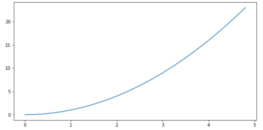
In the code above, we first define our data. We then call the figure function with the figsize parameter set to (10, 5). This creates a new figure with the specified width and height. We then plot our data on this figure.

How to Generate Subplots in Matplotlib plot function

Subplots allow for the creation of multiple plots within a single figure. The subplot function is used to create these, taking three arguments: the number of rows, the number of columns, and the index of the current plot. Let’s see how we can generate subplots:

x = np.arange(1, 5, 0.1)
y1 = np.log(x)
y2 = np.log2(x)
 
plt.subplot(2, 1, 1)
plt.plot(x, y1)
 
plt.subplot(2, 1, 2)
plt.plot(x, y2)
 
plt.show()

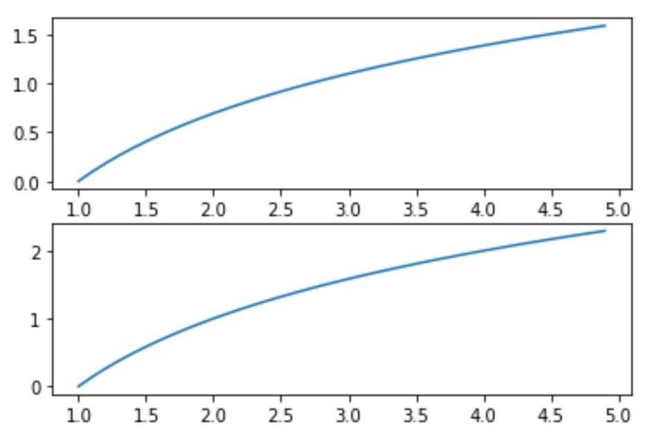
In the example code, we first define our data. We then call the subplot function to create the first subplot and plot the natural logarithm on it. We repeat the process for the base 2 logarithm.

How to Annotate Plots in Matplotlib plot function

Annotations can be added to plots using the annotate function. This function requires the text of the annotation and the point to which it refers. Let’s see how we can annotate a plot:

x = np.arange(0.1, 4, 0.5)
y = np.exp(-x)
 
plt.plot(x, y)
plt.annotate('Decay', xy=(1, 0.5), xytext=(2, 0.5),
             arrowprops=dict(facecolor='black', shrink=0.05))
plt.show()

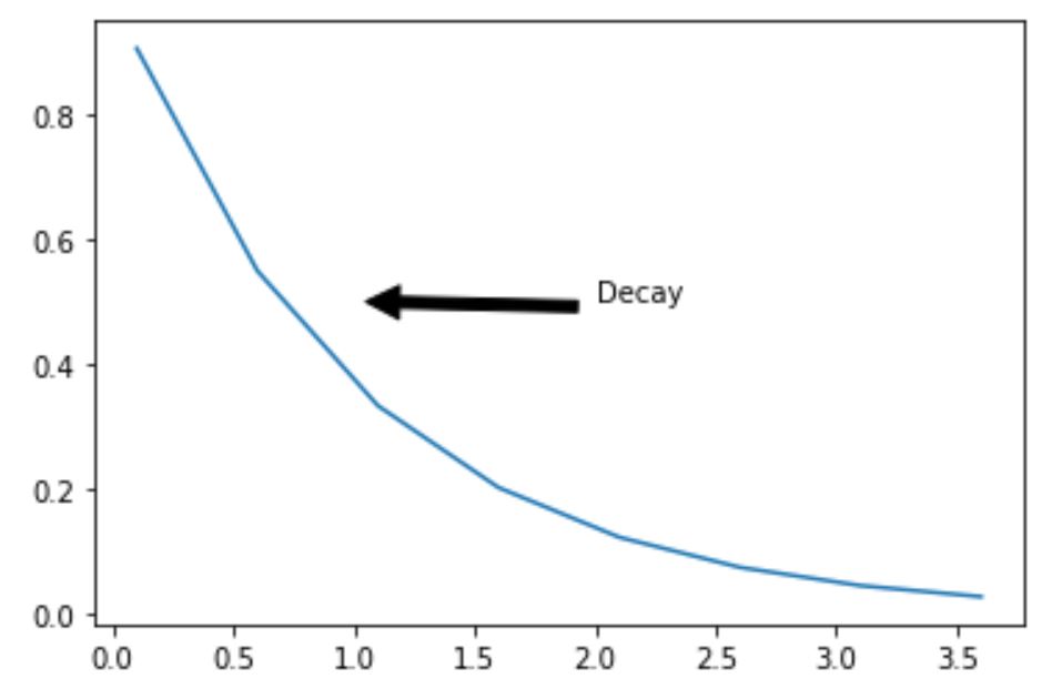
In the code above, we first plot an exponential decay function. We then call the annotate function to add an annotation. The xy parameter specifies the point that we want to annotate, and the xytext parameter specifies the location where the text will be placed. The arrowprops parameter is used to draw an arrow from the text to the point.

How to Modify Axes in Matplotlib plot

The axes of a plot can be modified using various functions such as xlim, ylim, xscale, yscale, xlabel, and ylabel. Let’s see how we can modify the axes of a plot:

x = np.arange(0, 5, 0.1)
y = np.sqrt(x)
 
plt.plot(x, y)
plt.xlim([0, 5])
plt.ylim([0, 2.5])
plt.xlabel('x')
plt.ylabel('sqrt(x)')
plt.show()

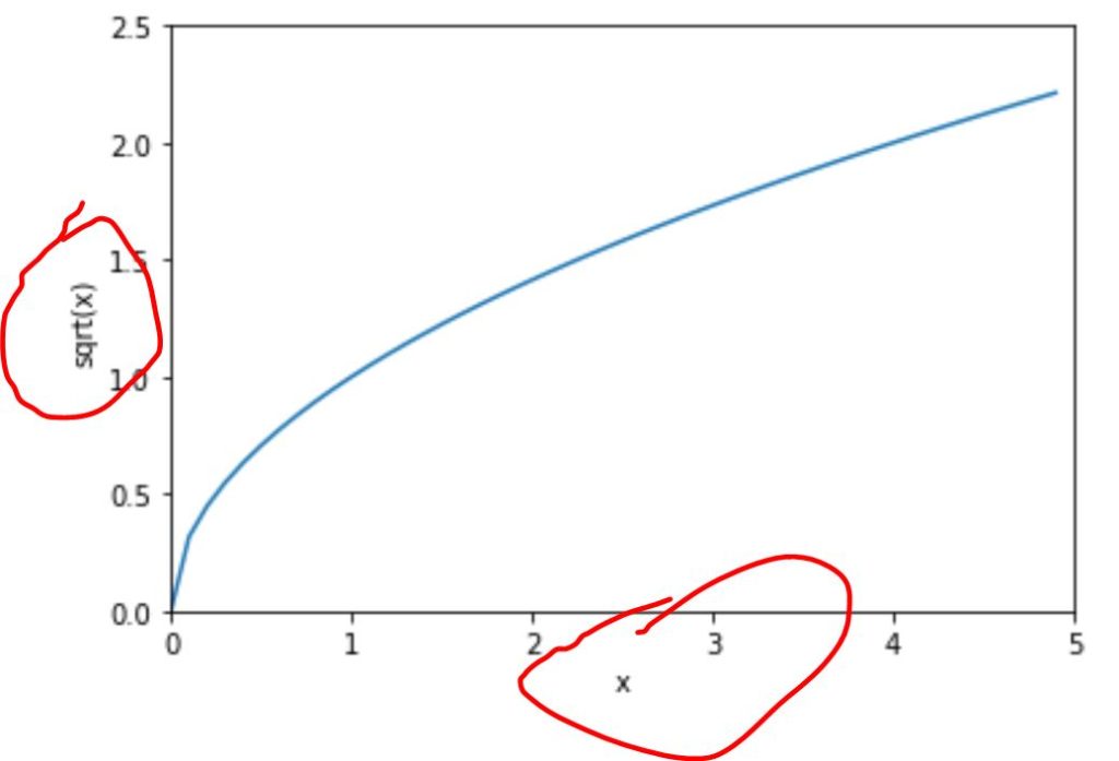
We first plot a square root function. We then call the xlim and ylim functions to set the limits of the x-axis and y-axis respectively. The xlabel and ylabel functions are used to set the labels of the x-axis and y-axis respectively.

How to Make Plots Interactive in Matplotlib plot

Matplotlib plots can be made interactive using the pyplot.ion() function. This allows for the plot to be updated in real-time. Let’s see how we can make a plot interactive:

plt.ion()
for i in range(50):
    y = np.random.gamma(2, size=1000)
    plt.hist(y, bins=30)
    plt.draw()
    plt.pause(0.1)
    plt.clf()

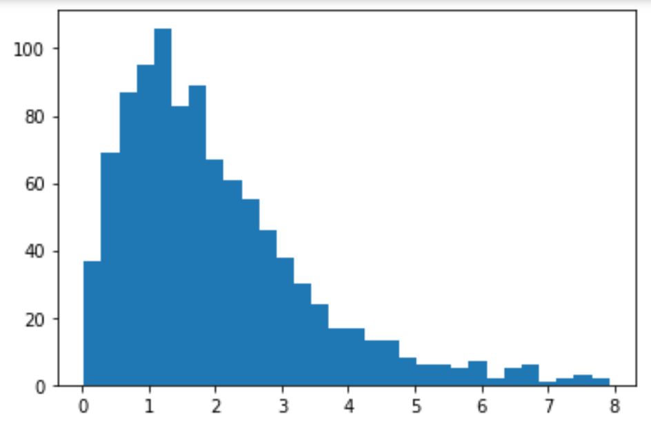
In the example code, we first call the ion function to turn on the interactive mode. We then enter a loop where we generate random data from a gamma distribution, plot a histogram of it, and then update the plot every 0.1 seconds. The clf function is called to clear the current figure after each iteration.

How to Group Bar Plots in Matplotlib

Grouped bar plots can be created by adjusting the x values of each bar. Let’s see how we can group bar plots:

labels = ['G1', 'G2', 'G3', 'G4', 'G5']
men_means = np.random.uniform(20, 40, size=5)
women_means = np.random.uniform(20, 40, size=5)
 
x = np.arange(len(labels))
width = 0.35
 
fig, ax = plt.subplots()
rects1 = ax.bar(x - width/2, men_means, width, label='Men')
rects2 = ax.bar(x + width/2, women_means, width, label='Women')
 
ax.set_ylabel('Scores')
ax.set_title('Scores by group and gender')
ax.set_xticks(x)
ax.set_xticklabels(labels)
ax.legend()
 
plt.show()

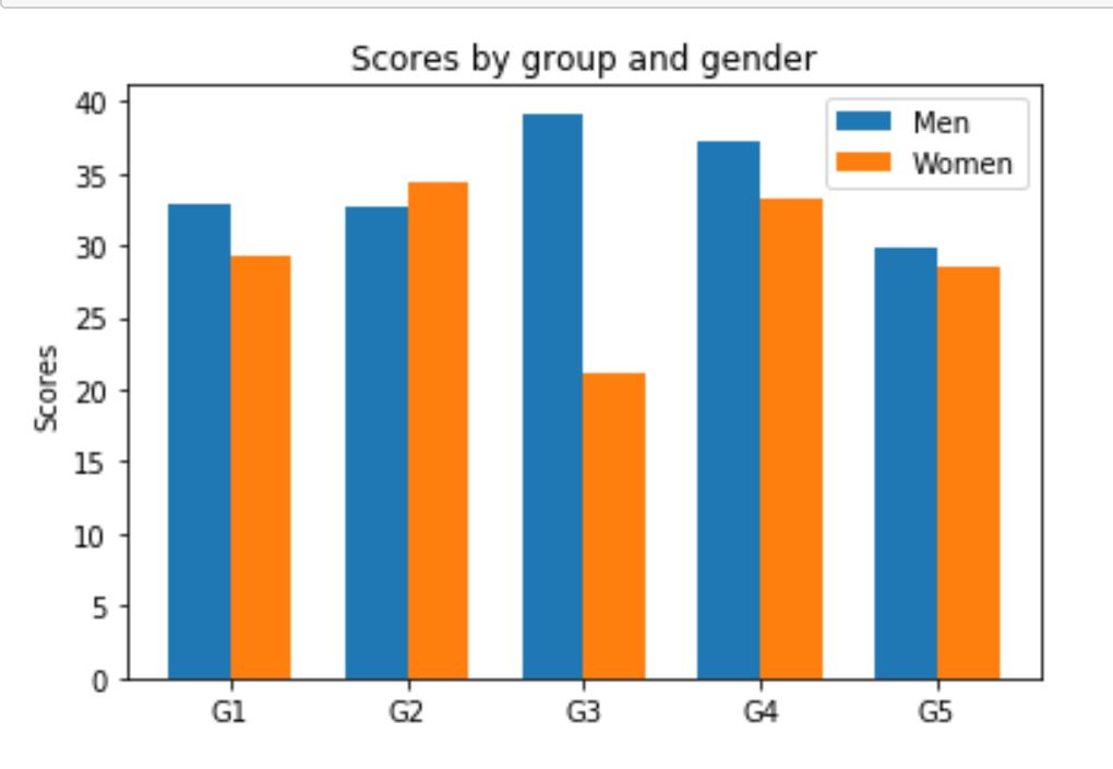
We first define our data and calculate the positions of the bars on the x-axis. We then create a new figure and axes, and plot the bars for men and women. The set_xticks and set_xticklabels functions are used to set the x-ticks and x-tick labels respectively. The legend function is called to add a legend. The show function is then called to display the grouped bar plot.

How to Plot Multiple Lines on the Same Graph

Multiple lines can be plotted on the same graph by calling the plot function multiple times before calling show. Let’s see how we can plot multiple lines on the same graph:

x = np.arange(0, 5, 0.1)
y1 = np.exp(x)
y2 = np.exp(-x)
 
plt.plot(x, y1, label='exp(x)')
plt.plot(x, y2, label='exp(-x)')
plt.legend()
 
plt.show()

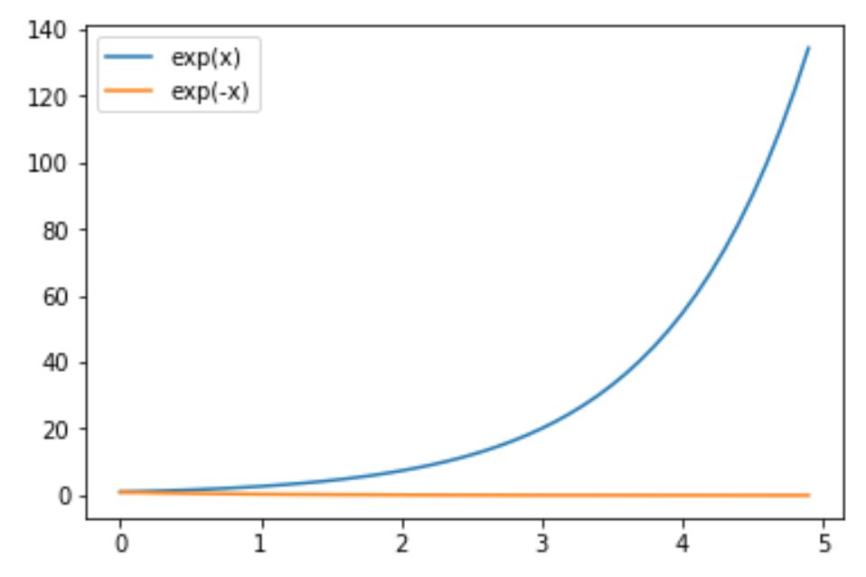
As you can see from the code, we first define our data. We then call the plot function twice to plot the exponential function and its inverse. The legend function is called to add a legend. The show function is then called to display the plot with the two lines.

How to Customize Line Styles and Markers in Matplotlib

Line styles and markers can be customized using various parameters in the plot function. Let’s see how we can customize line styles and markers:

x = np.arange(0, 5, 0.1)
y = np.power(x, 3)
 
plt.plot(x, y, linestyle='--', color='r', marker='o')
plt.show()

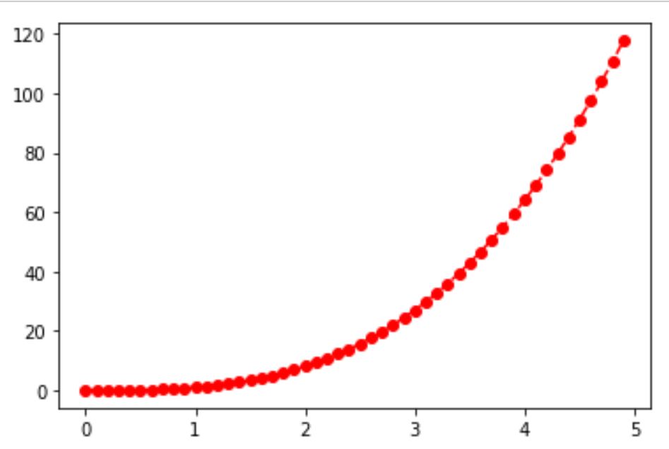
In the presented code, we first define our data. We then call the plot function with additional parameters to set the line style, color, and marker. The show function is then called to display the plot with the customized line style and markers.

How to Handle Large Datasets in plot function

When dealing with large datasets, it’s often useful to create a scatter plot instead of a line plot. Let’s see how we can handle large datasets with the plot function:

x = np.random.normal(size=10000)
y = np.random.normal(size=10000)
 
plt.scatter(x, y)
plt.show()

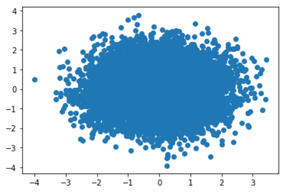
As shown in the code, we first generate two large arrays of random numbers from a normal distribution. We then call the scatter function to create a scatter plot. The show function is then called to display the scatter plot.

How to Plot Time-Series Data in Matplotlib

Time-series data can be plotted by passing datetime objects as the x values. Let’s see how we can plot time-series data:

import pandas as pd
 
dates = pd.date_range('20200101', periods=100)
data = np.random.randn(100).cumsum()
 
plt.plot(dates, data)
plt.show()

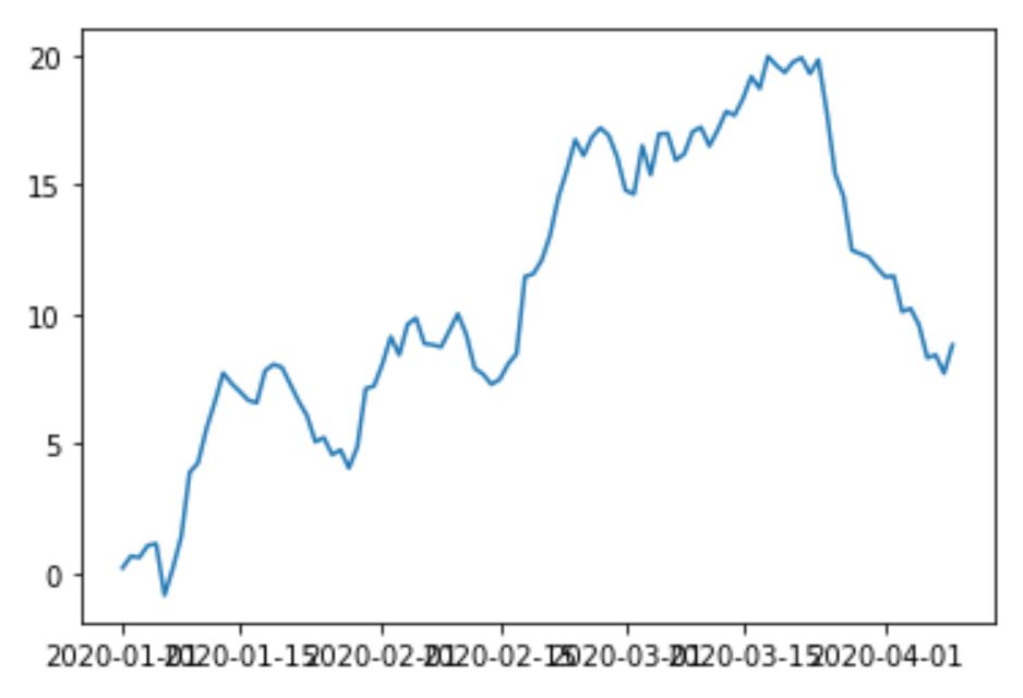
As indicated in the code snippet above, we first generate a range of dates and some random data. We then call the plot function to create a time-series plot. The show function is then called to display the time-series plot.

Summary about Matplotlib plot function

Matplotlib plot function is a versatile tool, capable of creating a wide variety of plots and charts. By understanding how to manipulate its parameters and utilize its features, one can create informative and visually appealing visualizations.

Whether you’re plotting simple line graphs, handling large datasets, or dealing with complex time-series data, Matplotlib has the tools to meet your needs. The ability to customize plots down to the smallest detail allows for a high degree of flexibility.

Moreover, the use of different data generator functions in each section demonstrates the adaptability of Matplotlib to various types of data. From mathematical functions like sine and cosine, to random data generation, Matplotlib can handle it all. In conclusion, mastering the plot function in Matplotlib opens up a world of possibilities. It is an essential tool for anyone looking to turn raw data into meaningful insights. So, dive in, explore its capabilities, and start crafting your own amazing plots and charts.